Introduction to Hydrology
- Topics and on line bibliography
- Introduction to Hydrology SCORM/AICC
- Intoduction PDF document
- Engineering Hydrology, Koutsoyiannis and Xanthopoulos (in Greek) file
- Hydrology in Practice, Elizabeth M. Shaw file
- Internet resources
- Web site about ancient Greek hydraulic works file
- Website with climatic diagrams and videos file
- Self Assessment Units
- Water variables calculations Quiz
- Introduction Quiz
- Climatic Quizz
- Surveys
- Gis Level Choice
- Familiarity with Hydrology Choice
Close the units before closing the water balance
A water balance can fail before any hydrological assumption is tested: the inputs may use different areas, periods or units. Make a small accounting sheet first. State a catchment boundary, a measurement period and one unit for each flux. The calculator below is an educational conversion exercise, not a model of a real river or a forecast.
Use the water-balance calculator as a separate practice after reading the lesson. Record your assumed quantities and units before calculating, then return to the module catalogue for the topic you need next. The calculator is a current editorial tool; it is not an original exercise attributed to the historical course.
Choose an accounting boundary
Imagine a fictional catchment with an area of 2 km². We use catchment-average precipitation, evapotranspiration and an outlet-flow volume for the same month. An average depth is not a reading from one rain gauge automatically representing the whole area. Record how any spatial average was obtained. Keep the month boundaries and time zone consistent across records.
USGS describes water budgets as accounting for water entering, leaving and being stored, including groundwater flows, withdrawals and transfers. Our teaching equation retains only precipitation P, evapotranspiration ET and outlet runoff Q: residual = P − ET − Q. It deliberately omits other exchanges. Call the answer a residual unless the omitted terms and measurement uncertainty have been addressed.
Convert depth into volume
One millimetre is 0.001 m and one square kilometre is 1,000,000 m². Multiplying them gives 1,000 m³. Therefore volume in m³ = depth in mm × area in km² × 1,000. A fictional 100 mm of rain over 2 km² represents 200,000 m³. This conversion does not depend on assuming that all rainfall becomes runoff.
Suppose ET is 40 mm and the month's outlet volume is 70,000 m³. Convert the volume back to an equivalent catchment depth: 70,000 ÷ (2 × 1,000) = 35 mm. The residual is 100 − 40 − 35 = 25 mm, or 50,000 m³. These numbers are invented for the exercise. The positive residual does not prove that an aquifer gained that much water.
A rate needs an interval
Do not put a discharge rate in m³/s directly into a monthly-volume field. If a constant rate is an explicit teaching assumption, multiply it by the number of seconds in the chosen interval. Real discharge varies; measured time series need appropriate integration and treatment of missing observations. Label estimated intervals rather than quietly replacing gaps with zero.
A negative residual is also a result to investigate. It may reflect storage depletion, an uncounted inflow, incompatible boundaries or uncertain measurements. Changing a sign to make the budget look balanced hides the question. Check snow and soil storage, groundwater exchange, abstractions and interbasin transfers as appropriate to the actual system.
Keep a unit audit beside the answer
Use the downloadable sheet to record source, period, area, original unit, conversion and uncertainty for each input. Keep the original values so another reader can reproduce the calculation. This modern editorial exercise accompanies the historical lesson; it does not announce an active degree programme or restore former enrolment arrangements.
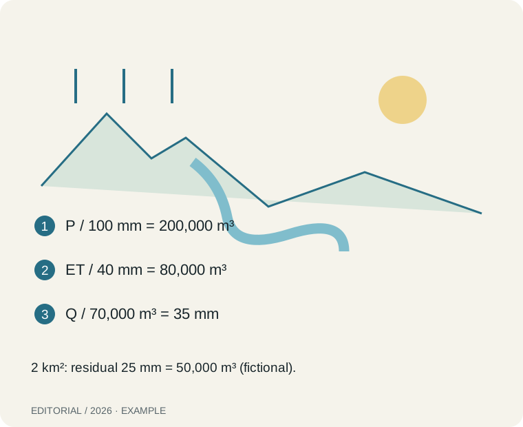
Text equivalent: P / 100 mm = 200,000 m³. ET / 40 mm = 80,000 m³. Q / 70,000 m³ = 35 mm. 2 km²: residual 25 mm = 50,000 m³ (fictional).
Try the local worksheet
Inputs stay in this page and are not sent or stored. Use anonymised examples. No account is needed.
This calculator needs JavaScript. Its inputs remain unavailable until it loads. The explanation and formula remain readable.
Download the blank worksheet and worked example ↓
Primary context and limits
From rainfall depth to catchment volume: keep the units visible
Rainfall depth and water volume answer different questions. Millimetres describe a layer over an area. Cubic metres describe a volume. Converting between them requires an area and a stated assumption about how the rainfall depth represents that area; it does not by itself estimate runoff.
The dimensional calculation
One millimetre is 0.001 metres. One square kilometre is 1,000,000 square metres. A uniform 1 mm layer over 1 km² therefore has a volume of 1,000 m³. For rainfall P in mm and area A in km², the illustrative precipitation volume is V = P × A × 1,000 m³.
Keep depth and area for the same boundary and period. A point rain-gauge reading may not represent a whole catchment. If you use an areal mean, record how it was derived. If you only have one gauge and no justification for representativeness, label the result an assumption-based estimate rather than a measured catchment total.
Three values you can reproduce
For a fictional catchment of 2 km² and an assumed uniform 100 mm depth over one specified period, precipitation volume is 100 × 2 × 1,000 = 200,000 m³. For a 0.5 km² area and 12 mm, the volume is 6,000 m³. For one hectare and 1 mm, first use 0.01 km²: the resulting volume is 10 m³.
These numbers are unit exercises, not observations of a real catchment. The diagram's volume is the rain falling on the boundary. It is not the volume reaching a drainage outlet, a flood peak, available drinking water or a tank size recommendation.
Write the check beside the result
- Boundary: name or draw the area, and state its original unit.
- Period: give start/end and the time basis used by the source.
- Depth: identify a point measurement, an areal estimate or a teaching input.
- Conversion: show depth in metres and area in square metres at least once.
- Interpretation: name the flux represented and what the calculation excludes.
Zero rainfall gives zero precipitation volume in this conversion; it does not establish that no water entered from upstream. A negative depth or a negative area should prompt a data check. Missing values remain missing. Do not substitute zero for an unavailable gauge record.
USGS explains the relationship between rainfall depth, area and volume. The metric examples here are independently calculated. The existing water-balance worksheet can place a precipitation estimate beside other fluxes only after their boundaries, periods and units are consistent. Losses, storage change and runoff need their own evidence.
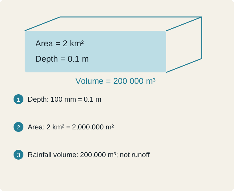
Text equivalent: Depth: 100 mm = 0.1 m → Area: 2 km² = 2,000,000 m² → Rainfall volume: 200,000 m³; not runoff
| Field | Completed example |
|---|---|
| Boundary and original area | Fictional 2 km² catchment |
| Period | One agreed teaching period |
| Depth source and representativeness | Assumed uniform 100 mm |
| Depth in metres | 0.1 m |
| Area in square metres | 2,000,000 m² |
| Volume / exclusions | 200,000 m³; runoff not calculated |
Blank worksheet and worked example ↓
Primary context: USGS: rain depth, area and volume · NIST: metric prefixes