Recovered from the public guest-access course page. Activities and file names describe the original teaching environment.
Wastewater Collection and Treatment
Introduction to process analysis and selection This lesson is of fundamental importance to wastewater treatment process design and environmental modelling in general. I have decided to split it in two lessons so next week there will be the second part of the lecture. I have offered a number of self assessment exercises to help you practice with concepts and notions.
Introduction to process analysis SCORM/AICC
Self assessment exercises
Fundamental quantities Quiz
Reaction rates Quiz
Handouts
Lecture - 4 pdf PDF document
Assignments
Assignment 4-1 Mass balance applications
Assignment 4.1 - Mass balance applications PDF document
Listed activities and handout names are preserved as text. Their original attachment files could not be recovered.
Concentration describes mass per volume; load also depends on the volume or flow passing through the boundary. Use the following fully fictional constant-flow example to keep units visible. It supplements the historical teaching page and is not a current course offering, a treatment design or a discharge-compliance assessment.
Define the substance, boundary and interval. Record concentration and the corresponding water volume or flow, including units and the sampling method. A single grab sample does not establish an average concentration over a changing event.
For this constant-value exercise, multiply concentration in mg/L by flow in L/s to obtain a mass rate in mg/s. Convert to g/s by dividing by 1000. A rate is not an event total until a duration is included.
Multiply that constant rate by the stated duration. For a varying real event, combine matched concentration and flow observations over the period using a justified method; do not multiply an unrelated average concentration by an unrelated average flow.
Compare concentrations, rates and totals in separate columns. Record what has not been measured. Neither the smaller concentration nor the calculated total alone proves a treatment is appropriate, safe, compliant or responsible for a change.
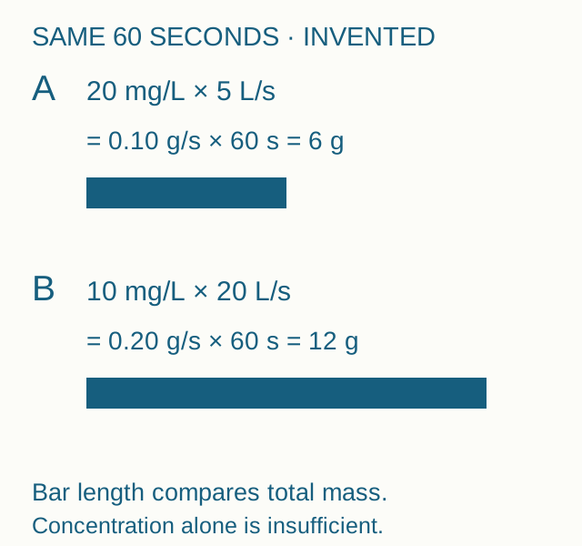
Case A: 20 mg/L times 5 L/s gives 0.10 g/s and 6 g in 60 seconds. Case B: 10 mg/L times 20 L/s gives 0.20 g/s and 12 g in 60 seconds. Lower concentration is accompanied by higher flow and mass rate.
Worked example and reusable record
Case A — invented
20 mg/L × 5 L/s = 100 mg/s = 0.10 g/s. Over a constant 60 s interval: 6 g.
Case B — invented
10 mg/L × 20 L/s = 200 mg/s = 0.20 g/s. Over a constant 60 s interval: 12 g.
Comparison
B has half A’s concentration, four times its flow and twice its mass rate. With equal durations, B also has twice the transferred mass.
Different duration
If B lasted only 15 s at those constant values, its total would be 3 g. The original equal-duration comparison would no longer apply.
Calculation record
Substance __; boundary __; concentration/unit/method __; matching flow/unit __; duration __; mass rate __; total __; unknown variation __.
EPA explains why concentration, volume and total load must be considered together when discussing stormwater controls. The original numbers here are arithmetic teaching fixtures, not measurements from EDUCATE, a field site or a treatment plant. Missing historical attachments remain missing.
Follow the water and the solids through a treatment plant
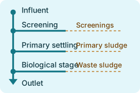
Draw two routes before deciding what a treatment stage achieved: the water route and the residuals route. This exercise uses a simplified municipal plant with primary settling and activated sludge. Actual plants can use other processes, include recycle streams and have additional treatment before discharge.
Mark the influent at the plant entrance. At screening, draw a separate branch for material removed by the screens.
Follow the liquid from primary settling into biological treatment and then secondary clarification. Record primary sludge at the first settling stage and waste sludge at the biological stage. Return sludge remains inside the selected plant boundary.
Mark a sampling point on the final effluent. Write the parameter, interval and units beside it. Keep the solids outlet and its measurement basis separate.
Worked check: suppose 12 kg of dry solids leave a primary settler in 1,000 L of sludge on a teaching day. The sludge carries 12 g of dry solids per litre. A student places this number beside the final water outlet. Move it to the sludge branch. The example supplies no final effluent result and no discharge limit.
Copy this record for any diagram: stage ___ · water enters from ___ · water continues to ___ · residual stream and destination ___ · sample point ___ · parameter and basis ___ · missing evidence ___.
Water continues to the outlet while screenings and sludge leave through separate routes.
Choose the average that answers the monitoring question
Before reporting an average concentration, name what receives equal weight: each observation, each second or each litre. Those averages can all differ. This fully synthetic two-interval exercise supplies constant concentration and flow within each interval; it is not a field dataset, a sampling protocol or a compliance assessment.
Start with the intervals
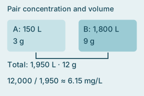
Interval A: 5 minutes, concentration 20 mg/L, flow 0.5 L/s. The duration is 300 s, so the volume is 150 L and transferred mass is 20 × 150 = 3,000 mg, or 3 g.
Interval B: 15 minutes, concentration 5 mg/L, flow 2 L/s. The duration is 900 s, volume is 1,800 L and transferred mass is 5 × 1,800 = 9,000 mg, or 9 g.
The complete event lasts 1,200 s, carries 1,950 L and transfers 12 g. Add matched interval masses first. Do not give the short interval the same duration or volume as the long one.
Three different concentration summaries
Equal-observation mean: (20 + 5) ÷ 2 = 12.5 mg/L. This gives the two listed observations equal weight, not the two volumes.
Time-weighted mean: (20 × 300 + 5 × 900) ÷ 1,200 = 8.75 mg/L. This answers a question about concentration across the stated clock time under the exercise’s constant-interval assumptions.
Volume-weighted mean: 12,000 mg ÷ 1,950 L ≈ 6.15 mg/L. This relates the total transferred mass to the total volume.
For this constructed dataset, mean flow is 1,950 ÷ 1,200 = 1.625 L/s. Multiplying that by the separate time-weighted concentration and duration gives 17.0625 g, not the correct 12 g. The concentration and flow vary together; averaging each separately loses the interval pairing.
Completed conclusion: “Total load 12 g; total volume 1,950 L; volume-weighted concentration about 6.15 mg/L; two constant synthetic intervals.” This is more reproducible than “average concentration 6.15” without its denominator and assumptions.
Blank record: substance ___; boundary ___; interval times ___; concentration and units ___; matching flow and units ___; interval volume/mass ___; missing observations ___; chosen weighting and question ___; result and rounding ___.
USGS’s stream-water sampling report describes flow-composite sampling as a distinct collection approach. A laboratory composite requires a justified sampling method; calculating a weighted mean afterward does not prove that real samples represented an event. Preserve the historical EDUCATE lesson and its missing attachments as they are.